Deep Learning series (Part 1): Introducing Artificial Neural Networks

In this new series of guides, you will essentially learn how to build your very own digital brain and teach it to recognize objects !

Image from brainstormingbox.org

Welcome to this brand-new series on Deep Learning in which we do a shallow deep-dive into understanding and building artificial neural networks (ANN), its sub-forms and close cousins. We will look at what neural networks can do, learn how to use and extend existing networks and how to build a simple one ourselves, and finally finish by building a more complex one that can classify images.
This series is split up into multiple different parts that build upon each other, so make sure you'll stick around for the other parts.

In this Part 1, we introduce the concept of ANNs. The actual building and usage of networks will follow in the subsequent parts. So, without further ado, let's get started!

What is an artificial neural network (ANN) ?

The terms Artificial Neural Network (ANN) and Deep Learning usually refer to the same thing.

The first neural networks were experimented with in the 1950s. During their history they have resurfaced several times, only to become uninteresting again.

Follow this link if you want to know more about the history of neural networks.

Over the last decade, ANNs have started a triumphant rise to the most powerful type of machine learning we know today. This is largely a consequence of Moore's Law and its implications for modern computers whose computational power has tremendously increased. Today, ANNs are mostly used for nonlinear problems tasks with complex input data such as:

recognizing objects in images
face recognition
speech recognition in a home assistant
automatic translation

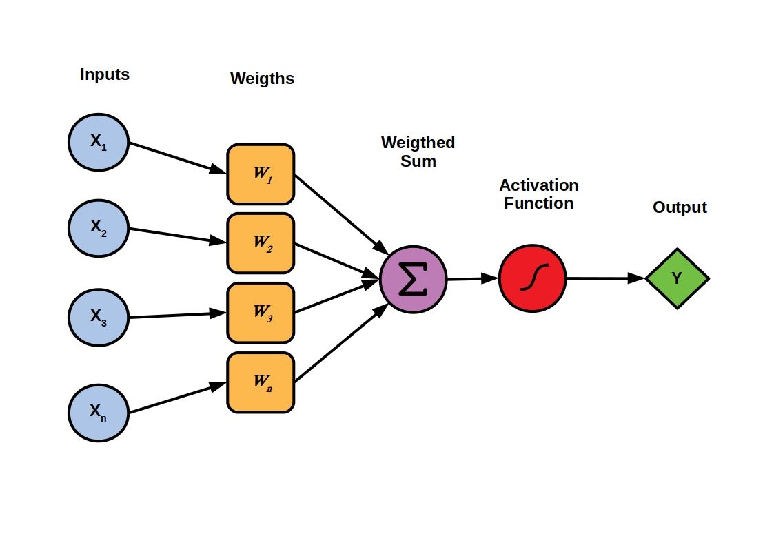
Mathematically, they are described by a single simple formula, the activation formula:

$\hat{y}= act(Xw+w_0)$

$y = \text{act}(\sum_{i = 0}^{n} w_ix_i + b)$

Where x is the input vector, w are the weights applied to x and w0 or b is the bias term.

We will look at what this function means functionally in the next section but for those familiar with linear systems, this function may already look familiar.

How does an ANN work ?

Neurons: the basic building blocks of ANNs

^ back to top ^

Any ANN contains at least one neuron (or perceptron). A neuron in an ANN borrows property logic from biological neurons (hence the name).

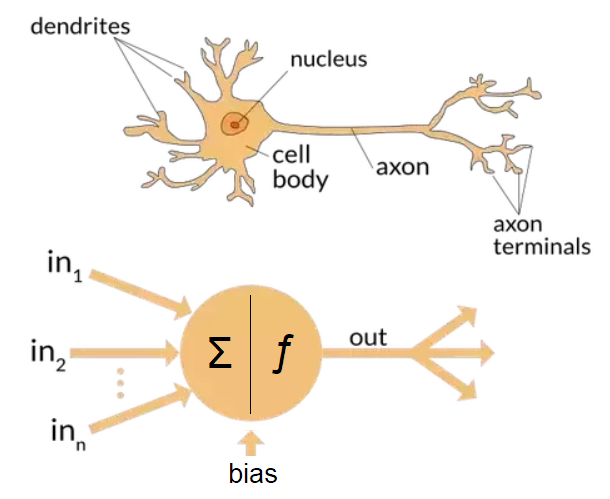
Follow this link if you want to know more about the relationship between neurons in ANNs and neurons in biology.

Neurons represent the most basic layer of any ANN. Each neuron receives at least a single input with a corresponding weight which contributes the neuron's activation function. For a single neuron, inputs and bias are multiplied with weights and then transformed by the activation function. In other words, the weights determine the influence of the input on the activation function as a weighted sum of all inputs, and so do biases except that they do not rely on a specific input.

A single neuron, also referred to as perceptron. Note that there is no bias in this illustration. Functionally, you can understand the bias as a combination of an input with a fixed weight. (image source: starship-knowledge.com)

Feed-forward Neural Networks

^ back to top ^

However, single neurons alone have limited use even if they have multiple inputs. The power of ANNs comes from population of neurons whose activation patterns can represent virtually any complex information. Populations of neurons are represented by and organized into networks.

For example, in one of the classic type of networks, the Feed-Forward Neural Networks (or Multi-Layer Perceptrons), many neurons are combined together into one or more hidden layers that feed into an output layer to form the network. In such networks, information strictly flows from the input to the intermediate layers (i.e. any number of hidden layers) to the output layer. This can be illustrated as follows:

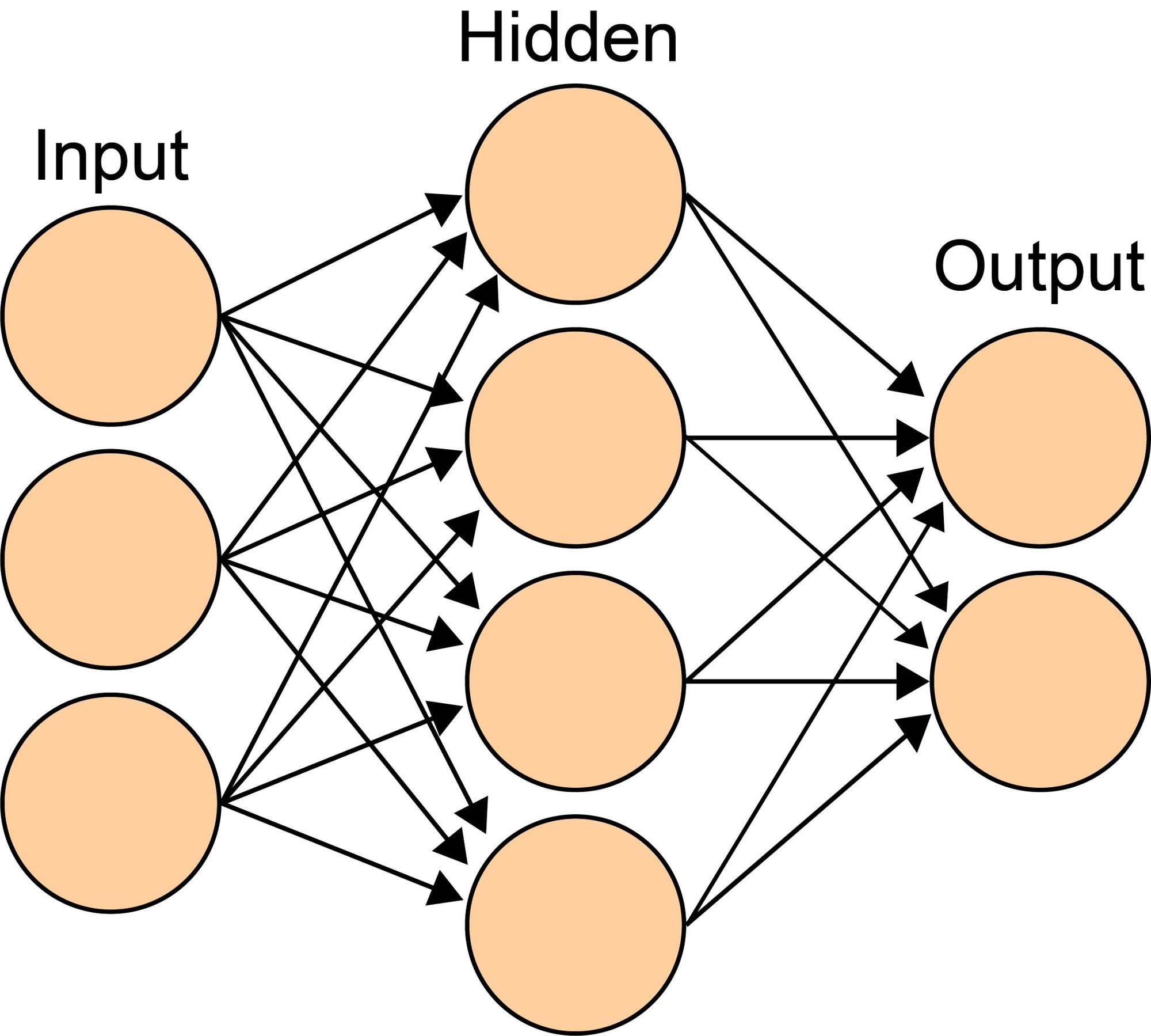
Schematic of a Feed-Forward Neural Network (image source: Wikipedia)

A note on terminology: we call each layer in between our input and output layer a hidden layer. In addition, weights to the output layer sometimes get referred to as outer weights while all other weights are referred to as hidden or inner weights. Each and any of the layers consists of one or more nodes (depicted as round circles in the above illustration) which is just another term for neuron. That means the above illustration shows a feed-forward neural network with an input layer containing three nodes, a single hidden layer containing four nodes, and an output layer with two nodes. In total, there are 12 hidden weights and 8 outer weights.

Hypothetically, a network with one hidden layer large enough is sufficient to learn anything. However, in practice, deep networks with multiple layers and other architectures are more efficient. In addition, every network has exactly one input layer, whose number of nodes is determined by the shape of the input data (plus an additional bias node in many networks), and exactly one output layer. The number of nodes of the output layer is determined by the chosen model configuration. We won't go into detail on this here but in short: if your network is a regressor, the output layer has a single node; if your network is a classifier it also has a single node unless your activation function is softmax, in which case it has as many nodes as you have unique class labels in your model.

Mathematically, neurons on top of neurons extend our equation from above by the hidden layer to:

$\hat{y}= act^{out}(act^{hidden}(X*w^{hidden}+w_0^{hidden})*w^{out}+w_0^{out})$

Recurrent Neural Networks

^ back to top ^

Now that we know what feed-forward neural networks are, we can also distinguish them from Recurrent Neural Networks (RNN). In general, the two different types of networks are fairly similar. However, the critical distinction lays in the types of feedback or more abstract how information flows within the network.

Remember that in feed-forward neural networks information flows strictly from input layers to the intermediate to the output layer. In that sense, feedback is hierarchical starting from the input layer leading ultimately to the output layer.
In contrast, in RNNs, we distinguish between three different types of feedback.

Direct feedback: output of a single neuron feeds the subsequent neuron or layer.
Indirect feedback: output of a single neuron is connected to a neuron of the preceding layers.
Lateral feedback: output of a single neuron is connected to another neuron of the same layer.

In other words, while neurons in feed-forward neural networks only use direct feedback or sequential mapping of information, neurons in RNNs use direct, indirect and lateral feedback or consider prior as well as subsequent information.

We will not go into detail regarding RNNs here in this post but in a different one at a later point.

Backpropagation: teaching your neural network

^ back to top ^

Now that we know the structure of an ANN, we can look at how it can be applied in order to solve a specific problem. It is clear, that the structure itself is only a framework. The real magic happens once we train the weights. Methodically, training the weights is achieved through backpropagation.

In a nutshell, improving the model through backpropagation entails an evaluation on how well the initial weights were performing on our training data set and based on the evaluation adjust the weights accordingly in order to increase the performance of our model. We iterate over this process until we achieve some threshold that is acceptable for us or until performance, according to our evaluation, no longer improves.

In that sense, backpropagation is an extension of the gradient calculation in the Gradient Descent algorithms. Arguably, Backpropagation is one of the most important algorithms today. Among other people, Geoffrey Hinton is responsible for making it popular. Like in Gradient Descent, the gradient of a loss function is used to calculate by how much to update the weights in the layers. The information about the gradient is then sent backwards through the network using the chain rule of differentiation (think calculus from your school time).

“The term back-propagation is often misunderstood as meaning the whole learning algorithm for multilayer neural networks. Backpropagation refers only to the method for computing the gradient, while other algorithms, such as stochastic gradient descent, is used to perform learning using this gradient.” — Goodfellow et al. (2016, p. 200)

Conceptually, backpropagation starts with the last parameter and works its way backwards to estimate all of the other parameters. The main idea of backpropagation is that when a parameter, such as a weight or bias is unknown, we use the chain rule of differentiation to calculate the derivative of our loss function with respect to that unknown parameter. Then, we set that parameter to some value (often times initially 0) and let gradient descent optimize the unknown parameter. Luckily, we can do this for all parameters in the model at simultaneously during backpropagation. Once we have hit the maximum number of iterations, or our threshold, we have optimized the entire network.

In the following, we outline this process step-by-step in a more in-depth way. For the purpose of the following explanation, we assume our network is a feed-forward network that contains one input layer, one hidden layer and one output layer. There are 3 input neurons, 4 hidden neurons, and 2 output neurons.

First, the neural network makes a prediction for a given input using randomly selected values for all parameters.
So we have an input vector x of size 3, and the weights between the input layer and the hidden layer are represented by a matrix W1 of size 3 x 4, and the biases at the hidden layer are represented by a vector b1 of size 4. The activations at the hidden layer h can then be calculated as follows:

$h = f(W1 * x + b1)$

Here, f is the activation function of the hidden layer neurons.

Next, let the weights between the hidden layer and the output layer be represented by a matrix W2 of size 4 x 2, and the biases at the output layer be represented by a vector b2 of size 2. The activations at the output layer y_pred can then be calculated as follows:

$y_{pred} = f(W2 * h + b2)$

Here, f is the activation function of the output layer neurons.
The error of the prediction is then calculated by comparing the predicted output to the known correct output value.
Let y be the known correct output value for the given input x. The error of the prediction can then be calculated using a loss function L, which measures the difference between the predicted output y_pred and the correct output y. A common choice for L is the mean squared error (MSE) loss function:

$L = \frac{1}{2} * \sum((y - y_{pred})^2)$

But other loss functions are also common, such as log-loss or sum of the squared residuals.
The error is then backpropagated, or passed backwards, through the network, starting at the output layer and working towards the input layer.
To backpropagate the error, we need to first calculate the gradient of the loss function with respect to the weights and biases in the network. This is done using the chain rule of differentiation.

For example, to calculate the gradient of the loss function with respect to the weights W2, we do the following:

$\frac{dL}{dW2} = \frac{dL}{dy_{pred}} * \frac{dy_{pred}}{dW2}$

Here, dL/dy_pred is the derivative of the loss function with respect to the predicted output y_pred, and dy_pred/dW2 is the derivative of the predicted output with respect to the weights W2. These derivatives can be calculated as follows:

$\frac{dL}{dy_{pred}} = -(y - y_{pred})$

$\frac{dy_{pred}}{dW2} = h$

Therefore,

$\frac{dL}{dW2} = -(y - y_{pred}) * h$

The gradients of the loss function with respect to the other weights and biases can be calculated in a similar manner.
As the error is backpropagated, it is used to update the weights of the connections between the neurons in the network. These weights are adjusted in such a way as to minimize the error of the prediction.
Once the gradients of the loss function with respect to the weights and biases have been calculated, the weights and biases can be updated using gradient descent.

For example, to update the weights W2, we do the following:

$W2 = W2 - \alpha * \frac{dL}{dW2}$

Here, alpha is the learning rate, which determines the size of the update to the weights.

The other weights and biases can be updated in a similar manner.
This process is repeated for each input in the dataset, and the weights are continually adjusted until the error of the predictions is minimized.
Once the error has been minimized, the neural network is considered to be trained and can be used to make predictions on new input data.

Now we know how train our neural network using backpropagation. Note that for more complex networks with many neurons and millions of inputs, stochastic gradient descent is applied simply because training the model would otherwise take too long. In stochastic gradient descent, a randomly selected subset of the data instead of the full dataset is used at every step of the gradient descent process.

What's next?

^ back to top ^

This was just an overview about the basics of ANNs. If you would like to know more, feel free to check out one of the videos I have linked at the end of this post.
In the next part, we will be building our very first super simple ANN and learn how to use and extend pre-trained ANNs.

See you in the next part!

UPDATE: Check Part 2 out here