Deep Learning series (Part 2): Building Artificial Neural Networks in Python using Tensorflow with Keras

 Welcome to the second part of our Deep Learning series. In this Part 2, we finally start building our own Artificial Neural Network (ANN) in Python. In three examples, I will show how to build your own model, use an existing model and extend an existing model to enable it to do more than for what it was initially designed for. To this end, we will use TensorFlow and one of its Python APIs Keras. We will start by briefly talking about what TensorFlow and Keras are before we move on to build and use ANNs in Python. Note that in order to follow this part it is essential to have grasped the main concepts of ANNs. If ANNs are new to you, make sure to check out Part 1 of this series!

What is Tensorflow?

 TensorFlow is an open-source software library for machine learning and artificial intelligence. It was developed by researchers and engineers working on the Google Brain team within Google's Machine Intelligence Research organization for the purposes of conducting machine learning and deep neural networks research, but the system is general enough to be applicable in a wide variety of other domains as well.

 At its core, TensorFlow is a mathematical library that allows you to perform efficient computations on arrays of data. These computations are often referred to as tensor operations, and the data being operated on is called a tensor. TensorFlow allows you to create computational graphs, which are a series of tensor operations arranged into a graph of nodes. The graph of nodes is then executed within a TensorFlow session, which allocates the necessary resources (such as memory and processing power) to perform the computations defined in the graph.

 One of the main benefits of using TensorFlow is that it allows you to easily train and deploy machine learning models on a wide variety of platforms, including desktop, mobile, and web applications. For example, you can use TensorFlow to train a model on a powerful desktop machine, and then deploy the trained model on a smartphone to make predictions on the go.

 In addition to its flexibility and portability, TensorFlow also offers a number of high-level APIs that make it easy to build and train machine learning models. For example, the TensorFlow Keras API provides a simple and powerful way to define and train neural networks, while the TensorFlow Estimator API offers a higher-level interface for training models on distributed platforms.

So, what can you do with TensorFlow? Here are just a few examples:

• Train and deploy machine learning models for image classification, natural language processing, and time series analysis
• Use deep learning to build self-driving cars, intelligent personal assistants, and language translation systems
• Use TensorFlow to optimize financial models and analyze stock market trends
• Use TensorFlow to develop medical diagnostic systems or predict disease outbreaks

 As you can see, the possibilities with TensorFlow are endless! Whether you are a seasoned machine learning engineer or a beginner just getting started, TensorFlow has something to offer for everyone.

What is Keras?

^   back to top   ^

 Keras is a high-level neural network API written in Python and capable of running on top of TensorFlow, CNTK, or Theano. It was developed with a focus on enabling fast experimentation and was released in 2015.

 One of the main benefits of using Keras is that it allows you to define and train deep learning models in just a few lines of code. It has a user-friendly interface that makes it easy to build and train complex neural networks, and it abstracts away much of the complexity of working with lower-level libraries such as TensorFlow.

 Keras is often used as the high-level API for TensorFlow, and it provides a convenient way to experiment with different model architectures and hyperparameters without having to dive into the details of TensorFlow. It also has a large and active community of users, which means that you can find plenty of online resources and support for using Keras.

 Overall, Keras is a powerful and user-friendly tool for building and training deep learning models that can be used in a wide range of applications. If you're interested in getting started with Keras, be sure to check out the official documentation and the numerous online tutorials and resources available.

How can we use Keras to build and use an artificial neural network in Python using Tensorflow?

^   back to top   ^

 Keras is designed with ease-of-use in mind, meaning that there is little necessary to do before you can start writing code to build and use an ANN in Keras. In fact, once you've installed TensorFlow (with pip install tensorflow) in your preferred virtual environment, you could start building a network in Keras. However, the one thing you should do first, is to think about the following three things:

1. The architecture of your model
2. The optimizers, metrics and loss function that should be used to train and evaluate your model
3. How many iterations (or epochs) you want to perform on how big of batch sizes of data.

More specifically, your model architecture is based on the following choice parameters:

• How many layers is your network going to have?
• What type of layer is each layer?
• How many nodes (neurons or units) are in each layer?
• Which activation function does each node use?

 If you are unsure about what these terms and decision entail, I highly recommend to go back to Part 1 of this series. Once you have made these decision, you can start to implement your model.

In the following, we will cover the following topics in three different examples:

1. Example: Build a model that can perform binary classification on fabricated non-linear data
2. Example: Use a pre-trained model that can classify image categories directly from image input
3. Example: Apply transfer learning to a pre-trained model so that it can do more than what it was originally trained to do

 The last two examples are based on examples by Sebastiaan Mathôt and an experiment of Chris Longmore.

Example 1:  
Training an artificial neural network to perform binary classification on fabricated non-linear data

^   back to top   ^

 To start out we will create and plot a made-up dataset using sklearn package. Note that using sklearn is not necessary. You could just as easy create data using other packages, such as numpy, or create it yourself from scratch.

# Imports
import pandas as pd
import numpy as np
import matplotlib.pyplot as plt
from sklearn.datasets import make_moons
from tensorflow import keras

# Create dataset using sklearn
X, y = make_moons(n_samples = 200, 
                  noise = 0.1,
                  random_state = 42
                 )
# Plot the dataset
plt.scatter(X[:, 0], X[:, 1], c = y)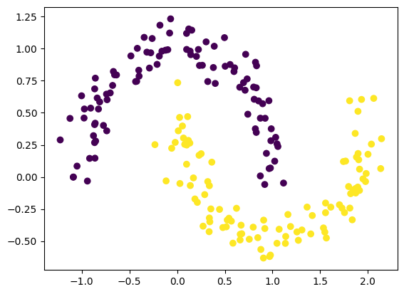

We see that the two individual classes in the data are non-linearly distributed.

Creating our model

^   back to top   ^

Now that we have our dataset, let's initialize our model object:

model = keras.models.Sequential()

 We can now start defining our first layer. For this example, we will build a very simple model with one input, one hidden and one output layer. Both the input and the hidden layer will have two nodes and are of the type Dense. The activation functions for our nodes will be sigmoid functions.

This is how we would implement our input and hidden layer using Keras:

model.add(keras.layers.Dense(input_dim = 2, # only for the first layer
                            units = 2, # number of neurons
                            activation = "sigmoid",
                            name = 'hidden_layer'))

 If we would have liked to add more hidden layers, we could simply do that by calling the add method of our model over and over again. In that way, we would sequentially add more layers to the network. Note that unless you are adding the first hidden layer, you will not need to define input_dim parameter. However, for this example, we would not like to add more hidden layers but finish the network by adding our second and last layer, the output layer:

model.add(keras.layers.Dense(units = 1,
                            activation = "sigmoid",
                            name = "output_layer"))

 Now, we are done with the model architecture and can check our model by calling model.summary().

 The model summary indicates that we have a total of 9 parameters. These parameters correspond to our two input nodes and a single bias node being fed to our two hidden layer nodes (that's 3 x 2 or 6 parameters), and the two hidden layer nodes and another single bias node feeding the output layer node (that's another 3 x 1 or 3 parameters).

Compiling our model

^   back to top   ^

 Since we have created a model, the next step is to compile the model. At this stage we need to input the loss function, optimizer and metrics. Check out the official documentation for more details on the possible parameters to Keras' modelling parameters

 The loss function typically describes the calculates the error, or the difference between the actual output and the predicted output. Different loss functions will give different errors on the same predictions. This choice has therefore a considerable effect on the performance of the model. For this example, let's choosebinary_crossentropy. This just means that the first output neuron is expected to be most active and the second the least active for 0 and vice versa for 1.

 It is given as a single parameter that describes the slope of the function in the gradient descent process. The closer the value to zero, the better the fit. That means we want to minimize our loss. Thus by choosing the loss function, we choose the minimization algorithm.

 The optimizer is the algorithm used to optimize the minimization process of our weights and the bias parameters during learning (see the chapter on backpropagation in Part 1 of this series). In a nutshell, the goal is to reduce the error which is achieved by modifying the weights and bias which is done by the optimization algorithm. This function repeatedly calculates the gradient or slope (i.e., the partial derivative) of the loss function with respect to weights and the weights are modified in the opposite direction of the calculated gradient until a local minimum is reached. A popular optimization algorithm is ADAM (Adaptive Moment Estimation), which is a more sophisticated stochastic gradient descent algorithm. It is fast and outperforms many other algorithms. We can also explicitly specify a learning rate (also called step size or alpha) for ADAM. Let's go with 0.3.

 Finally, we define the evaluation metric to assess the performance of our model after fitting. For this parameter, we simply go with binary_accuracy.

All together, this how we would implement model compilation in Keras:

model.compile(
              optimizer = keras.optimizers.Adam(learning_rate = 0.3),
              loss = keras.losses.binary_crossentropy,
              metrics = [keras.metrics.binary_accuracy] 
             )

Training our model

^   back to top   ^

 The next step is straight-forward: we fit, or train, our model. For this step, we need to define:

• The number of Epochs, or the number of times the data is fed into the model and the model is retrained. We go with 100 here.
• the batch size, or the number of samples per gradient update. Let's go with 32.
• the validation split, or the fraction of samples used as validation set (think train_test_split in sklearn). We choose 0.3.

This is the Keras implementation of model fitting:

model_history = model.fit(
                 X,
                 y,
                 epochs = 100, 
                 batch_size = 32, 
                 validation_split = 0.3)

Evaluating our model

^   back to top   ^

 In this step, we simply evaluate our model by observing the trend of the loss and accuracy. Keras provides us with a Python dictionary containing all the critical values so that we can plot directly, like so:

pd.DataFrame(model_history.history).plot()
plt.legend(bbox_to_anchor = [1, 1.02])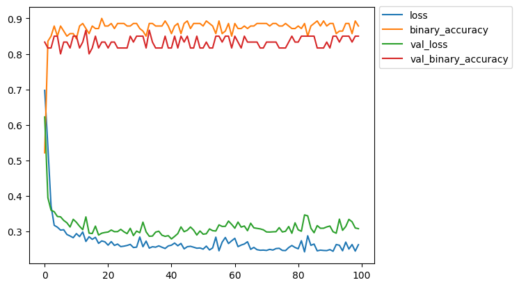

 We can say that, in spite of its simplicity, the model is doing fairly well. It is clearly not perfect and extensive training does not improve performance. But overall we can be confident to make a few predictions on data the model has not been trained on.

Predict unseen data

^   back to top   ^

 We first fabricate new data that, while different, is in its structure similar to the data we trained the model on. In reality, you assume that there are some commonalities between the data you have trained your model and the data you want to predict (in the future). Whether that assumption holds and what to do other than retraining your model when it does not is a discussion for another post.

So let's create some new data...

new_X, new_y = make_moons(n_samples = 200, 
                  noise = 0.1,
                  random_state = 2023 # different random state
                 )

... and predict the labels of that data using our previously trained model:

y_hat = model.predict(new_X)

Finally, let's plot the results of our prediction:

f = plt.figure(figsize=(15,6))
ax1 = f.add_subplot(121)  # row 1, col 2, index 1
ax2 = f.add_subplot(122)
x = np.linspace(0,4,1000)
ax1.scatter(new_X[:,0], new_X[:,1], c = new_y)
ax1.set_title('real classes')

ax2.scatter(new_X[:,0], new_X[:,1], c = y_hat)
ax2.set_title('predicted classes')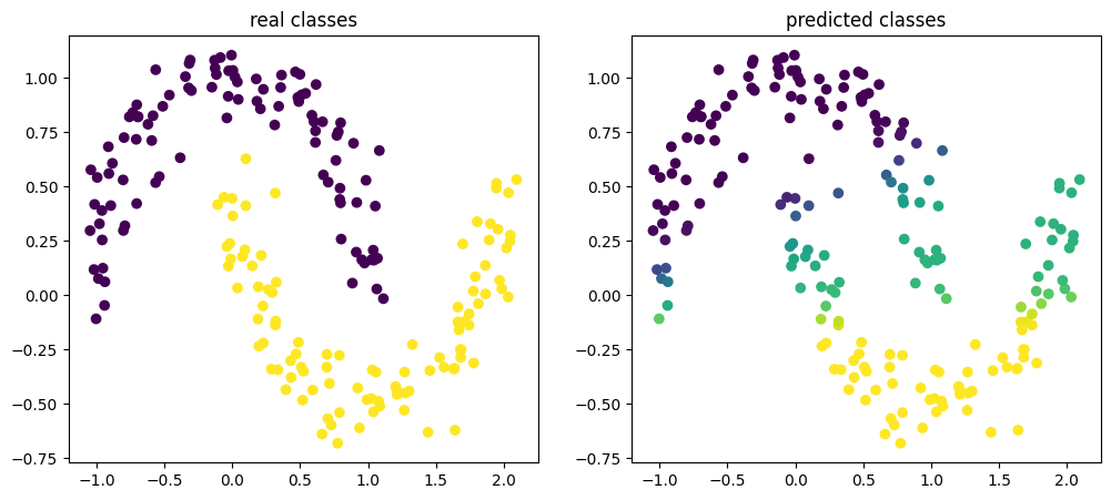

 We observe that the model is capable of capturing some of the labels correctly but overall does not perform extremely well. As it appears, it more or less fitted a straight line with a slightly positive slope to separate the classes. Clearly the architecture or the model parameters we chose are not optimal. Normally, we would have to go back to the drawing board and improve our model. For the purpose of this example, we are done and move on to the next example.

(Optional) Save (and load) the model for later use

^   back to top   ^

 Now that we have our model trained and evaluated and if we deem it to be worthy to be used again, we can save the model:

model.save("awesome_model.h5")

If we would want to reuse the model, we could simply load it with:

from tensorflow.keras.models import load_model

awesome_model = load_model("awesome_model.h5")

Example 2:
Use an artificial neural network to classify image categories directly from image input

^   back to top   ^

 Training and building your own model to perform well is an art in itself and it usually requires a lot of "good" data. Especially with image classification, accumulating good data and a lot of it is critical and training such a model can be extremely time consuming. So in this second example, where we use an ANN to classify image categories from an image input, we will use an already existing, pre-trained model that is capable of classifying pictures for us. In this example, we will make use of MobileNetV2.

But first things first, let's import all the packages we need:

from keras.applications.mobilenet_v2 import (
    MobileNetV2,
    preprocess_input,
    decode_predictions)
import numpy as np
from imageio import imread

Next, initialize our model with:

model = MobileNetV2(weights="imagenet")
model.summary()

 The model summary shows that the model is already built. We do not need to add any more layers. We could simply start using it. However, before we do that, we should pay attention to shape of the input layer InputLayer under Output Shape. We notice, the input shape is to be expected in 224, 244, 3, 0. In addition, we notice that our output layer, the predictions returns a vector of length1000. In other words, the output layer has 1000 nodes that are by the second-to-last layer called GlobalAveragePooling2D.

Loading an image to classify

^   back to top   ^

 Before we can start using our model, we need to load in the image we want to classify and bring it into a format MobileNetV2 can understand. So we will first load and preprocess the image, i.e. change it's resolution, because our image is likely not to match the resolution input the model was trained on.

We load our image, an image of an elephant, using the imageio package:

# Make sure the image is in the following format:
# (image_count, px height, px width, color channels)
data = np.empty((1, 224, 224, 3)) 
data[0] = imread("data/images/elephant.jpg")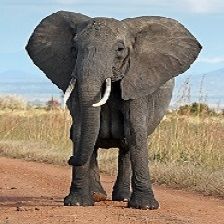

... preprocess it and make sure the shape is as we need it:

data = preprocess_input(data)
print(np.shape(data))

 The shape, or resolution, of our input image now matches the expected input shape required by MobileNetV2.

Classifying an image

^   back to top   ^

 Now that the image is in the right format for MobileNetV2, we can classify it using the model prediction, like so:

predictions = model.predict(data)
print(predictions.shape, predictions)

 This will output us the activations of the 1000 nodes, or predictions, of the output layer (see last paragraph of the first section in this chapter).

 Let's find the index of the node with the highest value or activation in our output layer:

# Return the activation of the most active node
highest_index = np.argmax(predictions, axis=1)[0]
print(predictions[0][highest_index])

 But this does not yet tell us as what the image was classified by the model. So let's get the label of the node with the highest activation:

for name, desc, score in decode_predictions(predictions, top=5)[0]:
    print("{}: {} ({:.2%})".format(name, desc, score))

 Looks like the classification worked. MobileNetV2 correctly classified the image as an elephant!

Example 3:
Transfer learning using an existing deep neural network

^   back to top   ^

 In the previous example, we used a pre-trained model to classify an image. However, in many cases, you might actually want to slightly modify a pre-trained model to do a task it was not originally trained to do while still benefitting from all the original training/learning that made it useful to begin with. So let's do that in this example. Here, we use the MobileNetV2 model again to classify an image but instead of classifying the type of animal, we want the model to identify whether the animal is male or female. For the purpose of this example, we will use images of cats.

Let's import all necessary packages, initialize MobileNetV2 and load the images:

# Import modules
from keras.applications.mobilenet_v2 import (
	MobileNetV2, 
	preprocess_input, 
	decode_predictions)
import numpy as np
from imageio import imread
from skimage.transform import resize
from keras import Model
from keras.layers import Dense

# Initialize the model
model = MobileNetV2(weights="imagenet")

# Load the images
data = np.empty((40, 224, 224, 3)) # bring it directly into the right format
# Note the order of operations matters! (i.e. first resize, then preprocessing won't work)
for i in range(20):
    im = imread("data/images/cat_images/f{:02d}.jpg".format(i + 1))
    im = preprocess_input(im) # preprocess the input to have pixel values between -1 and 1
    im = resize(im, output_shape=(224, 224))
    data[i] = im
for i in range(20):
    im = imread("data/images/cat_images/m{:02d}.jpg".format(i + 1))
    im = preprocess_input(im)
    im = resize(im, output_shape=(224, 224))
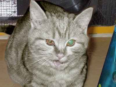
    data[i + 20] = im

This is a fairly representative image of all our cat images:

 Before we continue, let's make a sanity check to see whether the model recognizes all of our cat pictures:

predictions = model.predict(data)
for decoded_prediction in decode_predictions(predictions, top=1):
    for name, desc, score in decoded_prediction:
        print(f"- {desc} ({score*100:.2f}%)")

 Out-of-the-box classification of cats seems to work decently. Note: just because a score is pretty low does not mean the model is unsure about the classification category. Probabilities are just spread out across all possible categories and as we see here, there are plenty of different cat types that could be a classification of the cat image (i.e. it knows it's a cat just not as well which type of cat).

Modifying the model

^   back to top   ^

 There are various ways to modify a model. However, we will take all the layers of the existing model except the last, and then take the output of the second-to-last layer and connect it to our newly created output layer.

Let's look at the model again:

model.summary()

 Inspecting the whole summary output shows us that second-to-last layer, the GlobalAveragePooling2D has 1280 units/neurons and the last, the output layer (called predictions) has 1000.

Let's now connect the second-to-last layer to a new one for our cats:

cat_output = Dense(2, activation="softmax")
cat_output = cat_output(model.layers[-2].output) # output second-to-last layer
cat_input = model.input

# Create a model with the new layer
cat_model = Model(inputs=cat_input, outputs=cat_output)

 At this point, we do not want to compile and train the model because we would re-train the weights of all the already existing layers. We only want to train the newly created output layer and freeze the old layers.

for layer in cat_model.layers[:-1]:
    layer.trainable = False

Compiling the model

^   back to top   ^

 Next, we compile the model, like we did in the first example. We again choose ADAM as our optimizer, accuracy as our metric and as loss function sparse categorical cross entropy.

cat_model.compile(
    loss="sparse_categorical_crossentropy",
    optimizer="adam",
    metrics=["accuracy"],
)

Training the model

^   back to top   ^

 Since we have frozen MobileNetV2's original layers (i.e. made them untrainable) and compiled the model, we can now train it as we only train our newly added layer. However, we will have to create labels (i.e., for male and female cats) that we need for training:

labels = np.empty(40, dtype=int)
labels[:20] = 0 # male
labels[20:] = 1 # female

Now we can perform the training:

cat_model.fit(
    x=data,
    y=labels,
    epochs=20,
    verbose=2,
)

Generating predictions for the training data

^   back to top   ^

We are now ready to make predictions for our training data:

predictions = cat_model.predict(data)
# 40 images with 2 predictions (here the output nodes)
print(predictions.shape)

... find the most activate node of our two output nodes that is the most activated for each image:

np.argmax(predictions, axis=1)

 The model seems to be pretty quickly able to perfectly classify male and female cats since prediction accuracy is perfect (i.e., 1) even though the images are extremely similarly looking (i.e. this is a very difficult task). Is the model really that good or should we be suspicious of overtraining on our training data? In other words, always ask the question of what the model is actually classifying! Could it be that the model actually just memorized each of the images because there were so few?

Evaluating our model

^   back to top   ^

 The model we have built appears to be a classic case of an overfitted model. This highlights the need for a separate training and test sets to validate the predictions and how well your model generalizes to new, unseen data. So let's create these different sets very explicitly this time. We will use the first 15 images for male and female cats as training data:

training_data = np.empty((30, 224, 224, 3))
training_data[:15] = data[:15]
training_data[15:] = data[20:35]
training_labels = np.empty(30)
training_labels[:15] = 0
training_labels[15:] = 1

... and the last 5 images for male and female cats for validation:

validation_data = np.empty((10, 224, 224, 3))
validation_data[:5] = data[15:20]
validation_data[5:] = data[35:]
validation_labels = np.empty(10)
validation_labels[:5] = 0
validation_labels[5:] = 1

 We could now train our cat model again using the very same steps we have taken before. However, we need to create a new model instead of using the model we trained before because otherwise we would be cheating because the old model has already been trained on the validation images. So we create a new one and compile it.

cat_output2 = Dense(2, activation='softmax')
cat_output2 = cat_output2(model.layers[-2].output)
cat_input2 = model.input
cat_model2 = Model(inputs=cat_input2, outputs=cat_output2)
for layer in cat_model2.layers[:-1]:
    layer.trainable = False
cat_model2.compile(
    optimizer='adam',
    loss='sparse_categorical_crossentropy',
    metrics=['accuracy']
)

We are now ready to fit the new model:

# Split train and test data less verbose
cat_model2.fit(
    x=training_data,
    y=training_labels,
    validation_data=(validation_data, validation_labels),
    epochs=20,
    verbose=2
)

 We see indeed that the model is overfitting. How do we know that? We see that even after 20 epochs, validation accuracy barely improves above chance while training accuracy is perfect fairly quickly.

 If we think about what we have actually done, we realize that this makes sense: Telling apart female from male cats just based on frontal cat pictures seems to be hard especially when your data set is quite small.

In summary

^   back to top   ^

 The examples we looked at were clearly just simple toy examples. In practice, for building a ANN from scratch or extending an existing one, the real challenge is less to figure out how to code and build a network, but how to design its architecture such that it is capable of doing what you want it to do and to find enough good quality data to train that network (including "traditional" feature engineering).

 That was it for this part of the Deep Learning series. I hope you got an idea of how you can build a simple ANN in Python using TensorFlow and Keras on your own, and how you can use and expand upon already existing ANNs. In the next part of the Deep Learning series, we will take a look at how to build your own convolutional neural network (CNN). If you look at summaries of the models we used in this part, you will see that this won't be completely new to you as MobileNetV2 is actually a CNN.

So, see you in the next one!